Structural encoding describes how the “structure” of arrays is encoded into buffers and placed into a file. The choice of structural encoding places rules on how data is compressed, how I/O is scheduled, and what kind of data we need to cache in RAM. Parquet, ORC, and the Arrow IPC format all define different styles of structural encoding.
Lance is unique in that we have two different kinds of structural encoding that we choose between based on the data we need to write. In this blog post we will describe the structural encodings currently in use by Lance, why we need two, and how they compare to other approaches.
💡 📚 Series Navigation
This is part of a series of posts on the details we’ve encountered building a columnar file reader:
- Parallelism without Row Groups
- APIs and Fusion
- Backpressure
- Compression Transparency
- Column Shredding
- Repetition & Definition Levels
- Structural Encoding (this article)
What is Structural Encoding?
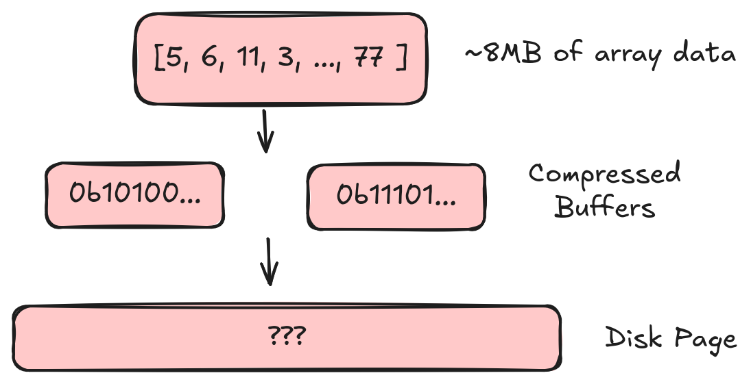
Structural encoding is the first step we encounter when we want to convert an Arrow array into an on-disk buffer. We start with a large chunk (~8MB by default) of array data. In the previous articles we described how we can take this array and convert it into a collection of compressed buffers. Now we need to take that collection of buffers and write it into a “disk page” (which is basically one big buffer in our file).
Structural Encoding Defines I/O Patterns
The structural encoding we choose is important because it defines the I/O patterns that we can support. For example, let’s look at a very simple structural encoding. We will write 2 bytes to tell us how many buffers we have, 4 bytes per buffer to describe the buffer length, and then lay out the buffers one after the other.
This is super simple and very extensible. It is, in fact, very similar to the approach used in Arrow IPC and ORC. It’s got a number of things going for it. However, there is one rather big problem. How can we read a single value?
Unfortunately, we know nothing about the makeup of the buffers. Are these buffers transparent or opaque? We don’t know. Is there some fixed number of bytes per value in each buffer? We don’t know. The only thing we can do is read the entire 8MB of data, decode and decompress the entire 8MB of data, and then select the value we want. As a result, this approach generally gives bad random access performance because there is too much read amplification.
💡 Read Amplification
Read amplification is a bit of jargon that describes reading more than just the data we want. For example, if we need to read 8MB of data to access a single 8-byte nullable integer, then we have a lot of read amplification; the 8-byte (plus one bit) read is amplified into 8MB.
Note: both Arrow IPC and ORC try to solve this problem a little. Arrow IPC is able to perform random access into the buffers if the data is uncompressed, but that requirement is not acceptable for us. ORC is able to chunk the values in a buffer so that only target chunks need to be read, but there is still considerable amplification.
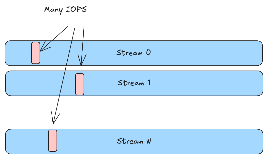
There is one further problem with the above approach. If a value is split into N different streams, then we need to perform at least N different IOPS to read that value. To use terms from a previous blog post, we are over-shredded and there is no zipping of values.
Structural Encoding Constrains Compression
Since the structural encoding is where we figure out which bytes we need to read from disk, it is highly related to several of the encoding concepts we described in earlier posts. Let’s review:
- Transparent compression (e.g., bit packing) ensures a value is not “spread out” when compressed. Opaque encoding (e.g., delta encoding) allows the value to be spread out but could potentially be more efficient.
- Reverse shredding (or zipping) buffers allows us to recombine multiple transparently compressed buffers into a single buffer. This avoids a value getting spread out but it requires extra work per-value to zip and unzip.
- Repetition and definition levels are a way to encode validity and offset information in a form that is already zipped. However, this form is not zero-copy from the Arrow representation and requires some conversion cost.
Each of these options has some potential trade-offs. In Lance, when we pick structural encoding, we end up solidifying these choices. As a result, in Lance, we don’t expect there to be a single structural encoding. It is a pluggable layer and there are already two implementations (technically three since we use a unique structural encoding for all-null disk pages).
Each is described further, but in summary, mini-block allows maximum compression but introduces amplification while full zip avoids amplification but limits compression.
| Structural Encoding | Transparency | Zipping | RepDef |
|---|---|---|---|
| Mini Block | Can be opaque | No zipping needed | Optional |
| Full Zip | Must be transparent | Zipping required | Mandatory |
Mini Block: Tiny Types Tolerate Amplification
Most columns in most datasets are small. Think 8-byte doubles and integers, small strings or enums, boolean flags, etc. When dealing with small data types, we want to minimize the amount of per-value work. In addition, when working with small values, a small amount of read amplification goes a long way. To handle these types, the mini-block structural encoding is used.
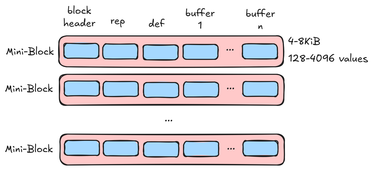
- Data is grouped into “mini blocks” and we aim for 1-2 disk sectors (4KiB-8KiB) per block.
- Blocks are indivisible. We cannot read a single value and must read and decode an entire block.
- We can use opaque encoding and avoid expensive per-value zipping.
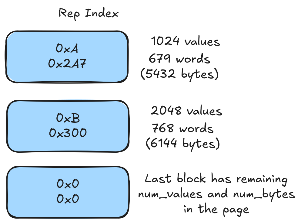
Repetition Index
In order to support random access, we need to translate row offsets quickly into block offsets and also be able to find the file offsets of the block. To support this, we store a repetition index for the mini-block encoding. This lightweight structure consists of 2 bytes per mini-block.
💡 Random Access Only
The repetition index does not need to be read when performing a full scan. However, it tends to be quite small, and avoiding it may not be worthwhile.
Mini Block vs. Parquet
Those of you who are familiar with Parquet will probably find mini-block encoding familiar. The concepts are basically the same. The repetition index is equivalent to Parquet’s page offset index (though more compact). The mini-block is equivalent to Parquet’s page (though our default size is much smaller). We can support any of the same encoding schemes that Parquet uses and, like Parquet, we require a small amount of read amplification.
Full Zip: Large Types Allow More Work Per Value
Lance needs to deal with multimodal data. Types like vector embeddings (3-6KiB/value), documents (10s of KBs/value), images (100s of KiB/value), audio (KBs-MBs/value), or video (MBs/value) do not fit into our normal database concept of “small values”. These types would end up giving us a single mini-block per value and, not surprisingly, this does not perform well!
To handle this, we use a different structural encoding for large data types, called full-zip encoding. During compression, we compress an entire 8MiB disk page, but we require transparent compression. This means we can take the resulting buffers (repetition, definition, and any value buffers) and zip them together. This allows us to read a single value without any read amplification.
- The entire 8MiB page is compressed at once (mini-block compresses individual blocks at a time) but we limit compression to transparent compression techniques (e.g., no delta or byte stream split)
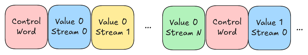
- Because compression is transparent, we know the start and stop of each compressed value and we can zip all value buffers together.
- Repetition and definition information are combined into a “control word” placed at the start of each value. If the value is a variable-length value (pretty typical), then this is also where we put the length of the value.
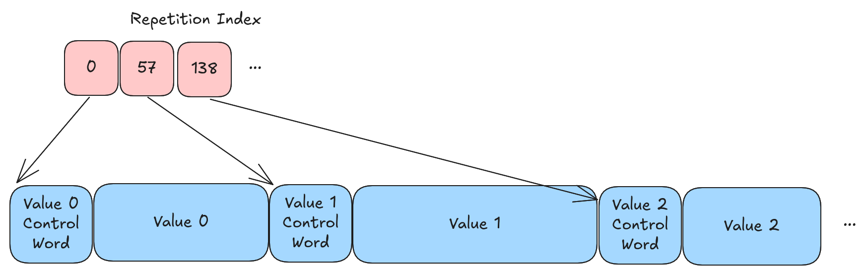
Repetition Index
Just like mini-block encoding, we need to have a repetition index to support random access. Unlike the mini-block encoding, this repetition index is quite a bit larger. The repetition index points to the start of each value (it’s very much like the Arrow offsets array in a binary or string data type). The resulting array of offsets can, of course, be compressed 😁
💡 Repetition Index
This repetition index is also only required when performing random access. It tends to be quite large and so skipping it during full scans can be beneficial.
Full Zip vs. Parquet
Parquet has no concept of full-zip encoding. When encoding large data types, you either have very large pages (e.g., 1MB) and lots of read amplification or you have a page-per-value. Page-per-value is quite similar to full-zip encoding. Value and structure buffers are co-located, the page offset index acts like a repetition index, etc. However, the overhead can be significant, both in terms of storage overhead (page descriptor overhead, the “number of values” part of the page offset index, etc.) and processing overhead (searching through the page offset index, page decoding overhead, etc.).
Does it Matter?
This is the part of the blog post where I share amazing benchmark results that show this new two-encoding approach blows the old-fashioned Parquet out of the water. I spent over a month doing detailed benchmarking, optimizing, experiment design, etc. It took a long time, and I had to overcome all sorts of noise and artifacts to eventually converge on something I feel represents reality. We wrote a whole paper on it, but I’ll summarize the findings here. When I was finally finished, I came to the somewhat disappointing answer that I still don’t know if all this is necessary.
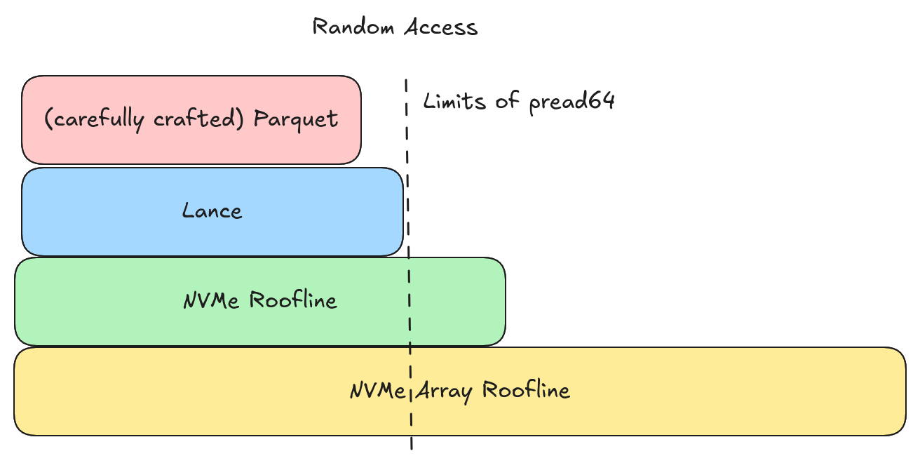
The Roofline Model
I started with a basic premise. Can I fully exploit an NVMe disk for both random access and full scans? To start with, I benchmarked an NVMe disk to figure out how many IOPS/s it can support. The answer was ~750K and we see an immediate drop-off as soon as we start requesting more than 4KiB per IOP. Note, this is much higher than cloud storage (cloud storage caps out around 10-20K IOPS/s).
Next, for full scans, I benchmarked the throughput of my disk. I was able to achieve a little over 3GBps.
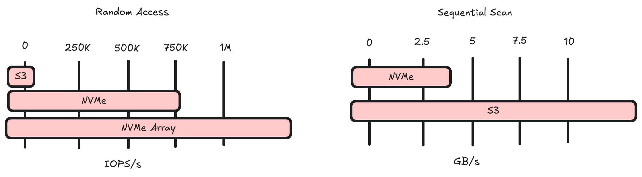
This makes the measure of success quite simple. Achieve 750K rows/second random access against an NVMe and 12.5GBps full scan performance against cloud storage.
💡 NVMe Array
For a long time my goal was to saturate an NVMe. Then I learned people build storage devices with an array of NVMe disks that can achieve millions of IOPS/s!
Making Parquet Sing
I was somewhat surprised by Parquet’s ability to handle random access. However, it did require some pretty complex configuration:
- I had to disable page-level statistics (once you start reaching page-per-value, these statistics will explode a file)
- I had to keep the number of row groups small (this is no surprise as row groups are inherently bad)
- I had to disable dictionary encoding (parquet-rs cannot cache dictionaries like Lance can)
- I had to make pages small (this was rather hard and I had to set a number of different settings like write batch size and page size and so on)
- I had to use the page offset index (this took up a lot of memory in page-per-value cases)
- I had to make sure to use the row selection API (e.g., Parquet’s equivalent of the take operation)
- I had to make sure to cache metadata (Lance needs to do this too, but it’s more automated)
- I had to use synchronous I/O (more on this later)
Making Lance Sing
I just used Lance’s default configuration (ok, I did have to resort to synchronous I/O and bump up the default page size 😇, more on this later).
Results
Both Parquet and Lance are able to come quite close to maximizing the IOPS of a single NVMe (can hit ~400K values/second random access), but we hit non-format limitations (e.g., syscall overhead) before we get there and we need a better I/O implementation.
💡 Parquet can do Random Access?!
It often surprises people that Parquet can perform efficient random access, but the principles are solid. With the page offset index, we perform one IOP per value. LanceDB’s primary gripe with Parquet remains “row groups” and (for vector search ) the RAM required for the page offset index.
Lance is able to keep up with (or beat) Parquet at full scan speeds in all the scenarios I tested. This includes scenarios where Parquet is configured with large page sizes. So our design is indeed able to maximize both full scan performance and random access performance.
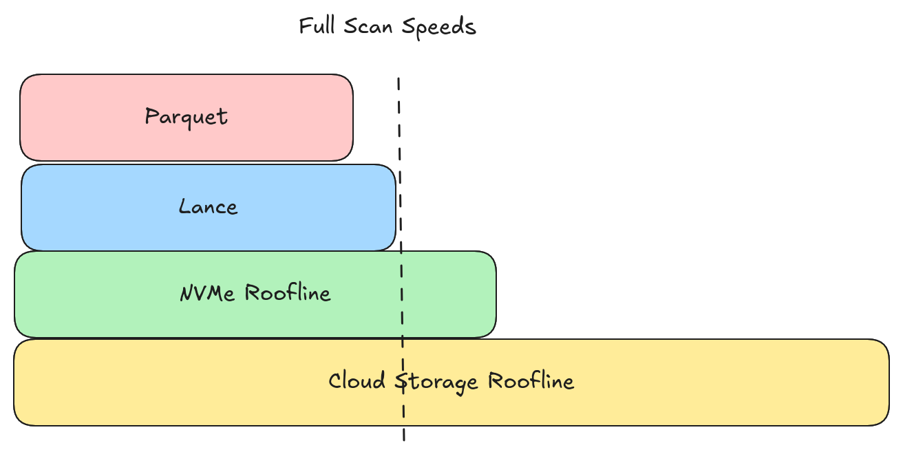
However, both Parquet and Lance fell short of the 3GB/s disk utilization roofline and well short of the 12.5GB/s cloud storage roofline. There is a fair amount of headroom available for improving full scan speeds.
One (not so) Minute Detail
There is one significant difference between Parquet and Lance that isn’t really related to performance but is somewhat critical if you happen to be implementing vector search 😉
If you have large fixed-width values that can’t be compressed (cough vector embeddings cough), then a full-zip structural encoding can be used without any repetition index. The equivalent Parquet would be page-per-value with a large page offset index which would incur significant RAM overhead. In other words, in this situation, a Parquet reader would need ~20GB of RAM per billion vectors, and Lance does not.
Conclusion
This post has covered a lot. We described the two kinds of structural encoding that Lance employs and discussed some of our benchmarking. Our design is flexible and is likely able to fully utilize an NVMe’s random access capabilities while matching Parquet’s full scan capabilities.
We are still well below the roofline performance that is possible. This is true for both random access and full scans. There is yet more work to do to improve the I/O scheduling, compression techniques, and overhead. I’m confident our flexible design will allow us to get there.
Want to Learn More?
LanceDB is building the data lake for AI & ML. Support for multimodal data, combining search and analytics, embracing embedded in-process workflows and more. If this sort of stuff is interesting, then check us out and come join the conversation on Discord or Github and we’d be happy to talk to you!
Appendix: Lessons Learned
You can probably skip the following sections unless you are the kind that really wants to know the details 😄
Random Access
Lesson 1: simple async I/O is too slow. With asynchronous I/O, both Parquet and Lance capped out around 50K reads/second. For Lance, at least, the problem is the time it takes to switch things between threads.
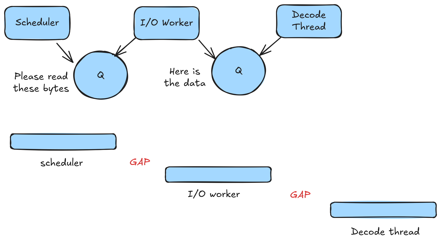
There are gaps while we wait for a thread to be notified, wake up, and grab the next item from the queue. These gaps only lasted a microsecond or less. When it comes to full scans, this is negligible. When it comes to random access, however, this is too expensive (a 1-sector read is only 1-2 microseconds). For the remainder of my experiments, I switched to synchronous I/O, though that has its own limitations.
Lesson 2: pread64 doesn’t cut it. Once on synchronous I/O, both Parquet and Lance were able to reach around 400K reads/second. This is surprisingly close to our roofline but doesn’t quite reach it. It turns out the bottleneck at this point is syscall overhead. For these experiments, we were using pread64 and the overhead of each call was simply too large.
Next Steps: io_uring. Both of the above problems should be solvable with io_uring. We would have asynchronous I/O without gaps (technically it’s a sort of semi-synchronous I/O) while also avoiding syscall overhead. In fact, Lance’s scheduler is pretty well suited for io_uring, so I think it should be a straightforward lift. The main obstacle has been that 400K IOPS is actually pretty good and we haven’t needed to get much faster yet, so it’s hard to prioritize this work.
Full Scans
For the next task, I wanted to make sure that Lance’s full scan performance could match Parquet and, even better, saturate S3’s bandwidth. Once again, I was somewhat disappointed.
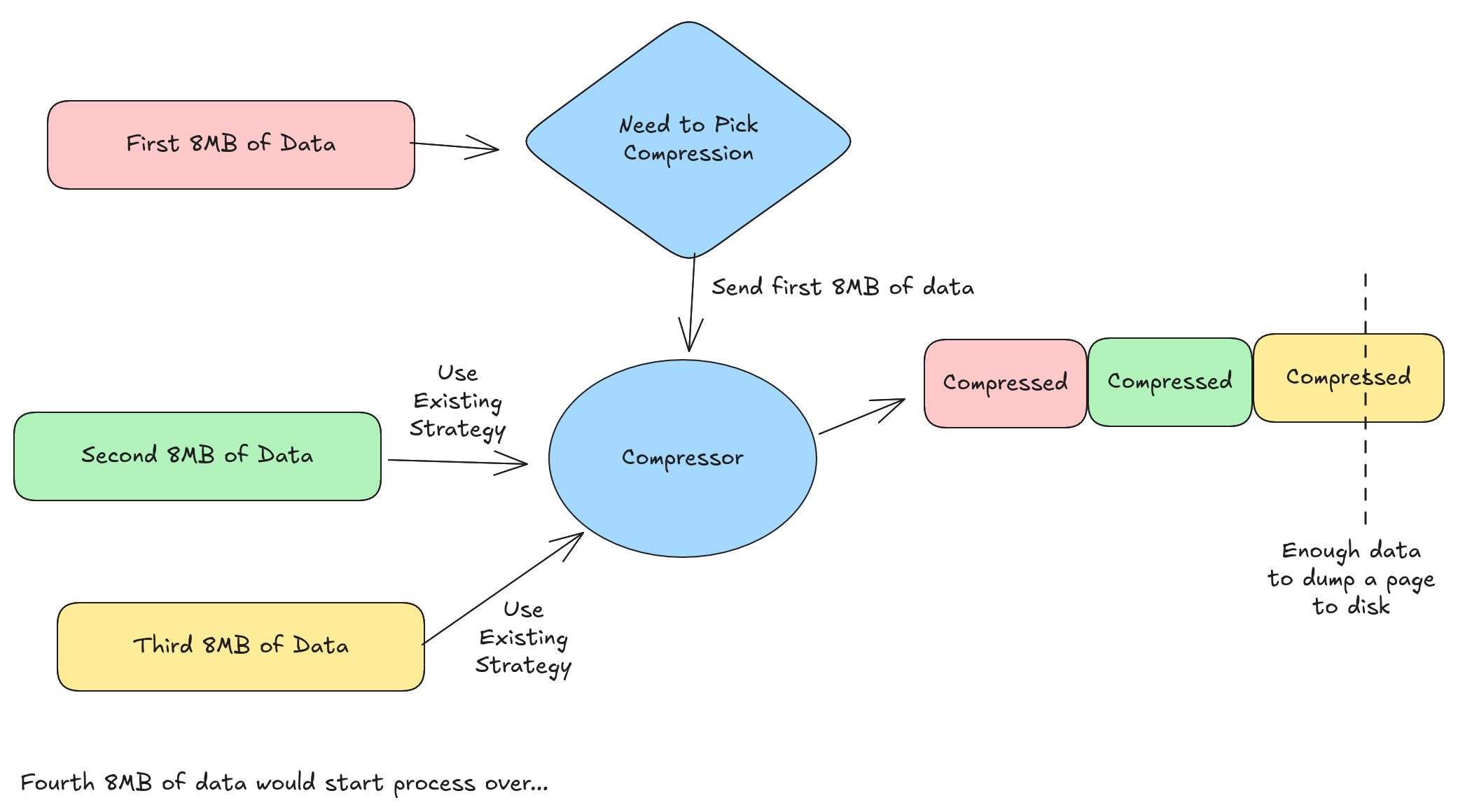
Lesson 3: Need rolling compression. In order to saturate S3 bandwidth, we need to make many (64-128) large (8-16 MB) parallel I/O requests. This is the rationale behind Lance’s default page size of 8MB. Unfortunately, the way a Lance column writer is currently implemented is as follows:
- Accumulate 8MB of uncompressed data
- Pick the best compression strategy to use
- Compress the data and write a page
The end result, when the data is highly compressible, is that pages might be much smaller than 8MB. In the future, I’d like to adopt some kind of “rolling” compression where we pick a compression strategy and create a compressor when we have 8MB of uncompressed data, and then keep feeding the compressor data until the compressed page is greater than 8MB. For my experiments, I was able to bump up the default page size to work around this limitation.
Lesson 4: Need better compression for larger values. Compression worked really well for small values (integers, names, labels, etc.). However, when we tried our compressors on large string values (code, websites) where each value was tens of kilobytes or more, we didn’t love the results. Both code and websites should be highly compressible, but our current FSST implementation was not very effective. I suspect it is an artifact of the way we are using it (or a bug) and not a limitation in FSST.
For simplicity, I switched to LZ4. LZ4 did give me good compression, but then the decompression speed was surprisingly not quick enough to keep up with the disk’s bandwidth. Our decompression speeds fell below what LZ4 benchmarks typically advertise, so I think there is some work to do there. One problem is that, in order to make LZ4 transparent (remember, these are large values and so we need transparent encodings), I needed to resort to LZ4-per-value, and I don’t know if the LZ4 implementation has a lot of per-call overhead that I need to find a way to avoid.
In-Memory Results
All of the above experiments were carefully designed to make sure that the data we were loading was not cached in memory already. This ensures we are truly testing I/O and that we have good I/O patterns. However, we did perform some results against in-memory data and there is some good evidence that the different structural encodings have significantly different performance patterns. Continuing these experiments to get a fuller picture of how the various formats do against in-memory data would be some interesting future work.