LanceDB WikiSearch: Native Full-Text Search on 41M Wikipedia Docs

It’s not about the vectors. It’s about getting the right result.

As developers take their RAG and search apps to production, they want three things above all: precision, scale, and simplicity. In this article, we introduce WikiSearch , our flagship demo that delivers on all these fronts, and illustrate how you can build scalable search systems using LanceDB.

WikiSearch is a search engine that stores and searches through real Wikipedia entries. The demo showcases how to use LanceDB’s full-text and hybrid search features to quickly find relevant information in a large dataset like Wikipedia.

Building the Wikipedia Search Engine

Here’s a closer look at the steps involved in building WikiSearch , from preparing the data to performing advanced queries.

Step 1: Data Preparation

We start with a subset of the Wikipedia dataset. The data is pre-processed and cleaned to ensure it’s in a consistent format. Each document in our dataset has a title and text field, which we’ll use for semantic and full-text search, respectively. There are a total of ~41M entries in the dataset.

Step 2: Embedding Generation & Ingestion

To enable semantic search, we first need to convert our text data into its vector representations. This is done by generating vector embeddings, which are numerical representations of the text that capture its underlying meaning. We use the popular sentence-transformers library for this task. The resulting vectors allow us to find conceptually related content, even if the exact keywords don’t match.

from sentence_transformers import SentenceTransformer

model = SentenceTransformer('all-MiniLM-L6-v2')
embeddings = model.encode(df['title'])

Here are the key performance metrics we achieved across an 8-GPU cluster:

Step 3: Creating the LanceDB Table and Indexes

With our data prepared and embeddings generated, the next step is to store everything in a LanceDB table. A LanceDB table is a high-performance, columnar data store that is optimized for vector search and other AI workloads. We create a table with columns for our title, text, and the vector embeddings we just created.

import lancedb
import pandas as pd

db = lancedb.connect("~/.lancedb")
table = db.create_table(
    "wikipedia",
    data=pd.DataFrame({
        "title": df['title'],
        "text": df['text'],
        "vector": embeddings
    })
)

To ensure our searches are fast and efficient, we need to create indexes on our data. For this demo, we create two types of indexes:

• A vector index on the vector column, which is essential for fast semantic search.
• A Full-Text Search (FTS) index on the text column, which allows for quick keyword-based searches.

# Create a vector index for semantic search
table.create_index(
    "vector",
    index_type="IVF_PQ",
    num_partitions=256,
    num_sub_vectors=96
)

# Create a FTS index for keyword search
table.create_fts_index("text")

Step 4: Performing Queries

Now that our data is indexed, we can perform various types of queries. LanceDB’s unified search interface makes it easy to switch between different retrieval techniques.

• Full-Text Search (FTS) is your classic keyword search. It’s perfect for finding documents that contain specific words or phrases.
• Vector Search goes beyond keywords to find results that are semantically similar to your query. This is powerful for discovering conceptually related content.
• Hybrid Search gives you the best of both worlds. It combines the results of both FTS and vector search and then re-ranks them to provide a more comprehensive and relevant set of results. This is often the most effective approach for complex search tasks.

Here are examples of how to perform each type of search using LanceDB’s intuitive API:

Full-Text Search:

fts_results = table.search("ancient civilizations").limit(5).to_pandas()

Vector Search:

query_vector = model.encode("famous landmarks")
vector_results = table.search(query_vector=query_vector).limit(5).to_pandas()

Hybrid Search:

text = "history of space exploration"
vector = model.encode(text)
hybrid_results = table.search(query_type="hybrid")\
    .vector(vector)\
    .text(text)\
    .limit(5)\
    .to_pandas()

Analyzing the Query

To help debug search issues and optimize performance, LanceDB provides two helpful methods : explain_plan and analyze_plan. This gives you a structured trace of how LanceDB executed your query.

Figure 5: Explain query plan

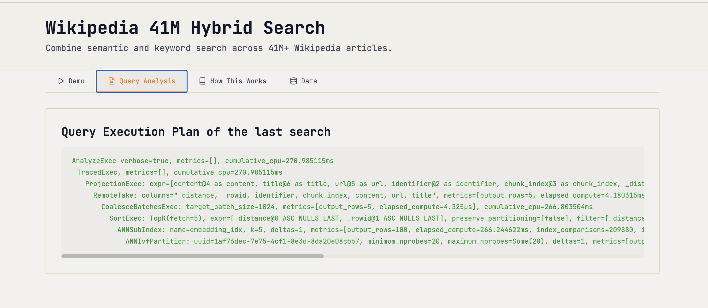
Running analyze_plan on the table with the FTS/vector index tells the following:

• Which indexes were used (FTS and/or vector) and with what parameters
• Candidate counts from each stage (text and vector), plus the final returned set
• Filters that applied early vs. at re‑rank
• Timings per stage so you know where to optimize

The WikiSearch Demo

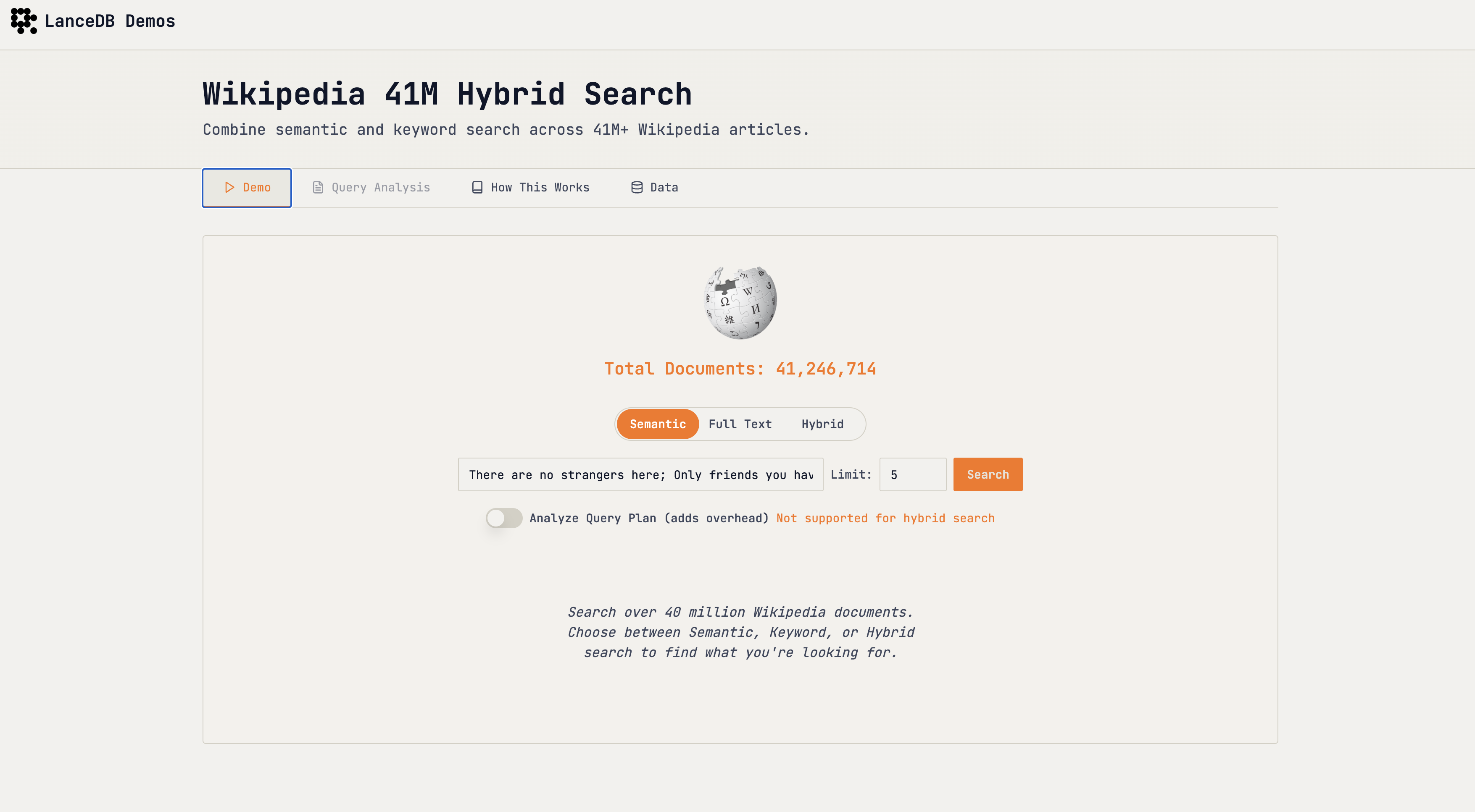
Want to know who wrote Romeo and Juliet? Give it a spin!

The demo lets you switch between semantic (vector), full-text (keyword), and hybrid search modes. Try comparing the different modes to see how they handle various queries and deliver different results.

Conclusions

This demo showcased what’s possible when you combine LanceDB’s native Full-Text Search with vector embeddings to create a powerful hybrid search solution.

You get precision via keyword matching, semantic relevance via embeddings, and the scalability and performance to handle massive datasets – all in one unified platform.