Most embedding models give you float32 vectors. That is precise, but wasteful. You pay in storage and query time. Scalar quantization can shrink the size, but not enough. Binary quantization can shrink it further, but at the cost of quality.
Until now LanceDB has relied on IVF_PQ (Inverted File with Product Quantization) as its default compression and search strategy. IVF_PQ works well in many cases, but comes with trade-offs: building PQ codebooks is expensive, re-training is required when data distribution shifts, and distance estimation can be slow. Learn more about index types in Indexing.
Today we are adding RaBitQ quantization to LanceDB. You now have a choice. IVF_PQ remains the default, but RaBitQ is available when you need higher compression, faster indexing, and better recall in high dimensions. See how this fits into vector search and hybrid search.
A 1024-dimensional float32 vector needs 4 KB. With RaBitQ and corrective factors the same vector takes about 136 bytes.IVF_PQtypically reduces this by 8–16x.
Why this matters for you
High-dimensional vectors behave in ways that seem strange if you are used to 2D or 3D. In high dimensions almost every coordinate of a unit vector is close to zero. This is the concentration of measure phenomenon often discussed in retrieval systems.
RaBitQ takes advantage of this. It stores only the binary "sign pattern" of each normalized vector and relies on the fact that the error introduced is bounded. The RaBitQ paper proves the estimation error is O(1/√D) (decreases proportionally to the inverse square root of dimensions), which is asymptotically optimal. In practice, the more dimensions your embeddings have, the more RaBitQ gives you for free.
💡 RaBitQ is most effective with embeddings of 512, 768, or 1024 dimensions. IVF_PQ often struggles more as dimensionality grows, making RaBitQ a strong complement.
What happens under the hood
When you index embeddings in LanceDB with RaBitQ your vectors are shifted around a centroid and normalized. They are snapped to the nearest vertex of a randomly rotated hypercube on the unit sphere. Each quantized vector is stored as 1 bit per dimension. Index creation is managed the same way as other vector indexes.
Two small corrective factors are also stored:
- the distance from the vector to the centroid
- the dot product between the vector and its quantized form
At query time your input—whether text, image, audio, or video—is transformed in the same way. Comparisons become fast binary dot products, and the corrective factors restore fidelity.
Formally, RaBitQ maps a vector v to a binary vector (vqb) and a hypercube vertex (vh) on the unit sphere:
where D is the number of dimensions. Each component is either a positive or negative value scaled by the square root of dimensions.
To remove bias, RaBitQ samples a random orthogonal matrix P and sets the final quantized vector to:
During indexing, for each data vector (v), we compute the residual around a centroid c, normalize it, map it to bits via the inverse rotation P-1, and store two corrective scalars alongside the bits:
- Centroid distance: 𝑑𝑐 =||𝑣 −𝑐||, which is the Euclidean distance from vector to centroid
- Inner product: 𝑑𝑠 =⟨𝑣𝑞,𝑣𝑛⟩, which is the dot product between quantized and normalized vectors
At search time, the query is processed with the same rotation to enable extremely fast binary dot products plus lightweight corrections for accurate distance estimates.

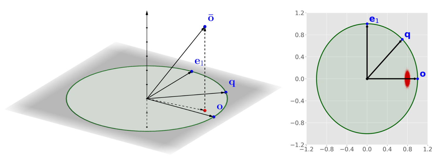
This figure shows the geometric relationship between a data vector o, its quantized form ¯𝑜, and a query vector q. The auxiliary vector e1 lies in the same plane. RaBitQ exploits the fact that in high-dimensional spaces, the projection of ¯𝑜 onto 𝑒1 is highly concentrated around zero (red region on the right). This allows us to treat it as negligible, enabling accurate distance estimation with minimal computation.
Difference with IVF_PQ: PQ requires training a codebook and splitting vectors into subvectors. RaBitQ avoids that entirely. Indexing is faster, maintenance is simpler, and results are more stable when you update your dataset.
Search in practice
With IVF_PQ you first partition vectors into inverted lists, then run PQ-based comparisons inside each list. With RaBitQ the comparison step is even cheaper: a binary dot product plus small corrections. Both approaches benefit from reranking with full-precision vectors.
Both approaches use a candidate set and re-ranking to ensure quality. But because RaBitQ's approximations are tight, you often need fewer candidates to hit the same recall.
For you this means recall above 95 percent with lower latency, even on large multimodal datasets on our test hardware.
💡 Always re-rank candidates with full precision vectors. IVF_PQ and RaBitQ both rely on approximation for candidate generation.
Research context: extended-RaBitQ
The RaBitQ paper also introduces extended-RaBitQ, a generalization to multi-bit quantization. Instead of limiting each coordinate to 1 bit, extended-RaBitQ allows for 2–4 bits per dimension. This reduces error further and can outperform product quantization under the same compression budget. For background on token-based search that pairs well with these methods, see Full‑Text Search.
⚠️ extended-RaBitQ is not yet available in LanceDB. We mention it here only as research context. It shows the trajectory of this work, and the same principles that make RaBitQ efficient at 1 bit can be extended to higher precision when needed.
Benchmarks

We tested IVF_PQ and RaBitQ side by side on two public datasets:
- DBpedia 1M (OpenAI embeddings)
- GIST1M (dense 960-dimensional vectors)
The tests were run on a consumer-grade PC:
- CPU: Intel 12400F (6 cores, 12 threads)
- Disk: 1TB SSD
- No GPU
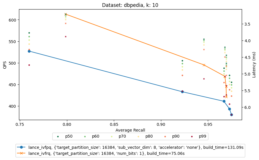
DBpedia (text embeddings, 768d)
| Metric | IVF_PQ | RaBitQ |
|---|---|---|
| recall@10 | ~92% | 96%+ |
| throughput | ~350 QPS | 495 QPS |
| index build time | ~85s | ~75s |
GIST1M (image embeddings, 960d)
| Metric | IVF_PQ | RaBitQ |
|---|---|---|
| recall@10 | ~90% | 94% |
| throughput | ~420 QPS | 540–765 QPS |
| index build time | ~130s | ~21s |

💡 On CPUs, RaBitQ already outperforms IVF_PQ on our test hardware. On GPUs the gap should widen further because RaBitQ operations are easier to parallelize.
IVF_PQ vs RaBitQ
When you use LanceDB today, the default quantization method is IVF_PQ. It works well for many workloads and gives you solid compression and recall. With RaBitQ now available, you have another option. The two approaches make very different trade-offs, especially when your vectors are high-dimensional or multimodal.
| Feature | IVF_PQ (default) | RaBitQ (new) |
|---|---|---|
| Compression ratio | 8–16x typical | Up to 32x |
| Index build time | Slower, requires codebook training | Faster, no training needed |
| Recall in high dimensions | Good but drops with >512d | Stays high, error shrinks with more dimensions |
| Query speed | Good, but PQ distance estimation is slower | Faster, binary dot products dominate |
| Update handling | Requires re-training if distribution shifts | No retraining needed, robust to updates |
| Best for | General workloads, balanced compression | Large multimodal datasets, high-dim embeddings |
What this means in practice is that you don't have to pick one forever. IVF_PQ remains a great default for balanced workloads. But if you are working with very large datasets, embeddings above 512 dimensions, or multimodal collections where precision matters, RaBitQ can give you higher recall, faster queries, and far smaller storage footprints. Because RaBitQ does not depend on heavy codebook training, you can also update your data more easily without re-training the index.
What you can do today in LanceDB
With IVF_PQ you already had scalable compression and fast ANN search. Now with RaBitQ you get an additional tool:
- Use IVF_PQ for general-purpose workloads where codebooks make sense
- Use RaBitQ when you want maximum compression, faster indexing, or higher recall in high dimensions
- Mix RaBitQ-S with other modalities for adaptive precision control
- Keep more embeddings online for RAG , multimodal search, and analytics
Proven and ready
RaBitQ is not theoretical. Elastic integrated it into their BBQ quantization feature. Tensorchord built a cost-efficient vector search service with it. Both show strong improvements in recall and speed compared to classical product quantization.
Now RaBitQ is available in LanceDB alongside IVF_PQ. You can choose the method that best fits your workload, and even switch as your dataset grows. If you're exploring LanceDB for the first time, check out our quickstart, the WikiSearch demo, and how this ties into the Multimodal Lakehouse.