Setup Real-Time Multimodal AI Analytics with Apache Fluss (incubating) and Lance

With the advent of the generative AI era, nearly all digital applications are integrating multimodal AI innovations to enhance their capabilities. The successful deployment of multimodal AI applications relies heavily on data, particularly for enterprise decision-making systems where high-quality, fresh data is critical. For instance, in customer service and risk control systems, multimodal AI models that lack access to real-time customer inputs will struggle to make accurate decisions.

Apache Fluss (incubating) addresses this need as a purpose-built streaming storage for real-time analytics.

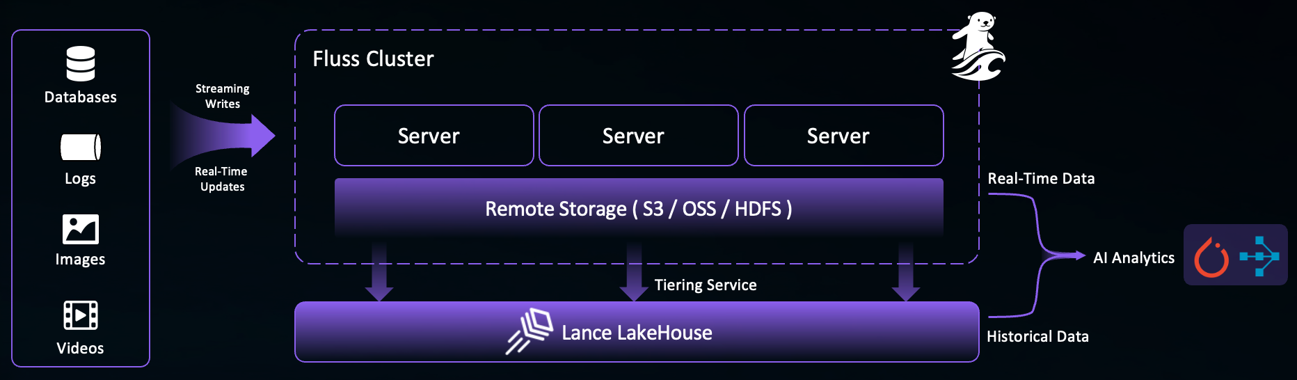
Serving as the real-time data layer for lakehouse architectures , Fluss features an intelligent tiering service that ensures seamless integration between stream and lake storage. This service automatically and continuously converts Fluss data into the lakehouse format, enabling the “shared data” feature:

• Fluss as the lakehouse’s real-time layer: Fluss provides high-throughput, low-latency ingestion and processing of streaming data, becoming the real-time front-end for the lakehouse.
• The lakehouse as Fluss’s historical layer: The lakehouse provides optimized long-term storage with minute-level freshness, acting as the historical batch data foundation for the real-time layer.

Complementing the Fluss ecosystem, Lance emerges as the next-generation AI lakehouse platform specialized for machine learning and multimodal AI applications. It efficiently handles multimodal data (text, images, vectors) and delivers high-performance queries such as lightning-fast vector search (see LanceDB ).

Combining Lance and Fluss unlocks true real-time multimodal AI analytics. Consider Retrieval-Augmented Generation (RAG) , a popular generative AI framework that enhances the capabilities of large language models (LLMs) by incorporating up-to-date information during the generation process. RAG uses vector search to understand a user’s query context and retrieve relevant information to feed into LLMs. With Fluss and Lance, RAG systems can now:

1. Perform efficient vector search on Lance’s historical data, leveraging its powerful indexes.
2. Compute live insights on Fluss’s real-time, unindexed streaming data.
3. Combine results from both sources to enrich LLMs with the most timely and comprehensive information.

In this blog, we’ll demonstrate how to stream images into Fluss, then load the data from the Lance dataset into Pandas DataFrames to make the image data easily accessible for further processing and analysis in your machine learning workflows.

MinIO Setup

Step 1: Install MinIO Locally

Check out the official documentation for detailed instructions.

Step 2: Start the MinIO Server

Run this command, specifying a local path to store your MinIO data:

export MINIO_REGION_NAME=us-west-1
export MINIO_ROOT_USER=minio 
export MINIO_ROOT_PASSWORD=minioadmin 
minio server /tmp/minio-tmp

Step 3: Verify MinIO Running with Web UI

When your MinIO server is up and running, you’ll see endpoint information and login credentials:

API: http://192.168.3.40:9000  http://127.0.0.1:9000 
   RootUser: minio 
   RootPass: minioadmin 

WebUI: http://192.168.3.40:64217 http://127.0.0.1:64217            
   RootUser: minio 
   RootPass: minioadmin 

Step 4: Create Bucket

Open the Web UI link and log in with these credentials. You can create a Lance bucket through the Web UI.

Fluss and Lance Setup

Step 1: Install Fluss Locally

Check out the official documentation for detailed instructions.

Step 2: Configure Lance Data Lake

Edit your <FLUSS_HOME>/conf/server.yaml file and add these settings:

datalake.format: lance

datalake.lance.warehouse: s3://lance
datalake.lance.endpoint: http://localhost:9000
datalake.lance.allow_http: true
datalake.lance.access_key_id: minio
datalake.lance.secret_access_key: minioadmin
datalake.lance.region: eu-west-1

This configures Lance as the data lake format, with MinIO as the warehouse.

Step 3: Start Fluss

<FLUSS_HOME>/bin/local-cluster.sh start

Step 4: Install Flink Fluss Connector

Download the Apache Flink 1.20 binary package from the official website . Download Fluss Connector Jar and copy it to Flink classpath <FLINK_HOME>/lib.

Step 5: Configure Flink Fluss Connector

The Flink Fluss connector utilizes the Apache Arrow Java API, which relies on direct memory. Ensure sufficient off-heap memory for the Flink Task Manager by configuring the taskmanager.memory.task.off-heap.size parameter in <FLINK_HOME>/conf/config.yaml:

# Increase available task slots.
numberOfTaskSlots: 5
taskmanager.memory.task.off-heap.size: 128m

Step 6: Start Flink

Start Flink locally with:

<FLINK_HOME>/bin/start-cluster.sh

Step 7: Verify Flink Running

Open your browser to http://localhost:8081 and make sure the cluster is running.

Launching the Fluss Tiering Service

Step 1: Get the Tiering Job Jar

Download the Fluss Tiering Job Jar .

Step 2: Submit the Job

./bin/flink run <path_to_jar>/fluss-flink-tiering-0.8.jar \
    --fluss.bootstrap.servers localhost:9123 \
    --datalake.format lance \
    --datalake.lance.warehouse s3://lance \
    --datalake.lance.endpoint http://localhost:9000 \
    --datalake.lance.allow_http true \
    --datalake.lance.secret_access_key minioadmin \
    --datalake.lance.access_key_id minio \
    --datalake.lance.region eu-west-1 \
    --table.datalake.freshness 30s

Step 3: Confirm Deployment

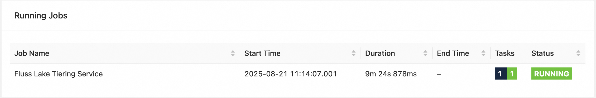
Check the Flink UI for the Fluss Lake Tiering Service job. Once it’s running, your local tiering pipeline is good to go.

Multimodal Data Processing

We’ll walk through a Python code example that demonstrates how to stream a dataset of images into Fluss, and subsequently load the tiered Lance dataset into a Pandas DataFrame for further processing.

Step 1: Create Connection

Create the connection and table with the Fluss Python client:

import fluss
import pyarrow as pa

async def create_connection(config_spec):
    # Create connection
    config = fluss.Config(config_spec)
    conn = await fluss.FlussConnection.connect(config)
    return conn

async def create_table(conn, table_path, pa_schema):
    # Create a Fluss Schema
    fluss_schema = fluss.Schema(pa_schema)
    # Create a Fluss TableDescriptor
    table_descriptor = fluss.TableDescriptor(
        fluss_schema,
        properties={
            "table.datalake.enabled": "true",
            "table.datalake.freshness": "30s",
        },
    )

    # Get the admin for Fluss
    admin = await conn.get_admin()

    # Create a Fluss table
    try:
        await admin.create_table(table_path, table_descriptor, True)
        print(f"Created table: {table_path}")
    except Exception as e:
        print(f"Table creation failed: {e}")

Step 2: Process Images

import os

def process_images(schema: pa.Schema):
	# Get the current directory path
	current_dir = os.getcwd()
	images_folder = os.path.join(current_dir, "image")

	# Get the list of image files
	image_files = [filename for filename in os.listdir(images_folder)
         if filename.endswith((".png", ".jpg", ".jpeg"))]

	# Iterate over all images in the folder with tqdm
	for filename in tqdm(image_files, desc="Processing Images"):
		# Construct the full path to the image
		image_path = os.path.join(images_folder, filename)

		# Read and convert the image to a binary format
		with open(image_path, 'rb') as f:
			binary_data = f.read()

		image_array = pa.array([binary_data], type=pa.binary())

		# Yield RecordBatch for each image
		yield pa.RecordBatch.from_arrays([image_array], schema=schema)

This process_images function is the heart of our data conversion process. It is responsible for iterating over the image files in the specified directory, reading the data of each image, and converting it into a PyArrow RecordBatch object as binary.

Step 3: Writing to Fluss

The write_to_fluss function creates a RecordBatchReader from the process_images generator and writes the resulting data to the Fluss fluss.images_minio table.

async def write_to_fluss(conn, table_path, pa_schema):
    # Get table and create writer‘
    table = await conn.get_table(table_path)
    append_writer = await table.new_append_writer()
    try:
        print("\n--- Writing image data ---")
        for record_batch in process_images(pa_schema):
            append_writer.write_arrow_batch(record_batch)
    except Exception as e:
        print(f"Failed to write image data: {e}")
    finally:
        append_writer.close()

Step 4: Check Job Completion

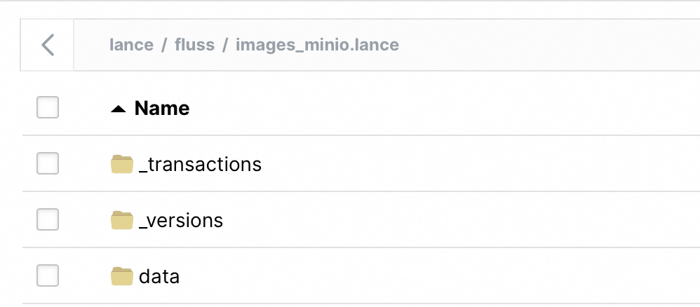
Wait a little while for the tiering job to finish. Then, go to the MinIO UI, and you’ll see the Lance dataset in your lance bucket. You can load it with Pandas using Lance’s to_pandas API.

Step 5: Loading into Pandas

While Fluss is writing data into Lance in real time, you can load from the Lance datasets in MinIO. At this point, you can leverage anything that integrates with Lance to consume the data in any ML/AI application, including PyTorch for training (see Lance + PyTorch integration ), LangChain for RAG integration , and LanceDB for hybrid search. You can also use Lance’s Blob API to have efficient, low-level access to the multimodal image data.

Here, we present a simple loading_into_pandas example to describe how to load the image data from the Lance dataset into a Pandas DataFrame using Lance’s built-in to_pandas API, making the image data accessible for further downstream AI analytics with Pandas.

import lance
import pandas as pd

def loading_into_pandas(table_name):
	dataset = lance.dataset(
        "s3://lance/fluss/" + table_name + ".lance", 
        storage_options={
            "access_key_id": "minio", 
            "secret_access_key": "minioadmin", 
            "endpoint": "http://localhost:9000", 
            "allow_http": "true",
        },
    )
    
    df = dataset.to_table().to_pandas()
	print("Pandas DataFrame is ready")
	print("Total Rows: ", df.shape[0])

Putting It All Together

If you would like to run the whole example end-to-end, use this main function in your Python script:

import asyncio

async def main():
    config_spec = {
        "bootstrap.servers": "127.0.0.1:9123",
    }
    conn = await create_connection(config_spec)
    table_path = fluss.TablePath("fluss", table_name)
    pa_schema = pa.schema([("image", pa.binary())])
    await create_table(conn, table_path, pa_schema)
    await write_to_fluss(conn, table_path, pa_schema)
    # sleep a little while to wait for Fluss tiering
    sleep(60)
    df = loading_into_pandas()
    print(df.head())
    conn.close()

if __name__ == "__main__":
    asyncio.run(main())

Conclusion

The integration of Apache Fluss (inclubating) and Lance creates a powerful foundation for real-time multimodal AI analytics. By combining Fluss’s streaming storage capabilities with Lance’s AI-optimized lakehouse features, organizations can build multimodal AI applications that leverage both real-time and historical data seamlessly.

Key takeaways from this integration:

• Real-time Processing: Stream and process multimodal data in real-time with sub-second latency, enabling immediate insights and responses for time-sensitive AI applications.
• Unified Architecture: Fluss serves as the real-time layer while Lance provides efficient historical storage, creating a complete data lifecycle management solution.
• Multimodal Support: The ability to handle diverse data types like images, text, and vectors makes this stack ideal for modern multimodal AI applications .
• RAG Enhancement: Real-time data ingestion ensures that RAG systems always have access to the most current information, improving the accuracy and relevance of multimodal AI-generated responses.
• Simple Integration: As demonstrated in our example, setting up the pipeline requires minimal configuration and can be easily integrated into existing ML workflows.

As multimodal AI applications continue to demand fresher data and faster insights, the combination of Fluss and Lance provides a robust, scalable solution that bridges the gap between real-time streaming and AI-ready data storage . Whether you’re building recommendation systems, fraud detection, or customer service chatbots, this integration ensures your multimodal AI models have access to both the timeliness of streaming data and the depth of historical context.