The Quest for One Million IOPS: Benchmarking Storage at LanceDB

Introduction

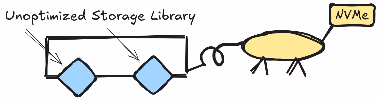
One of the main goals of the Lance file format (and our storage layer in general) is fast random access. As NVMe drives have become cheap and common the need for sequential reads has diminished. However, utilizing the full potential of these drives is a difficult task and exactly the kind of fun problem that engineers love to tackle. Recent NVMe drives can achieve millions of IOPS! However, it’s easy for applications to fail to utilize this potential. So I decided to take a crack at it and see just what it would take to utilize 1,000,000 IOPS. In this blog post I’ll explain how the journey went, but also explain how we benchmark random access and what it means to us.

Random Access is Typically Search

Random access is almost never a user requirement. Fetching the Nth row of a table is not typically the end-goal of an application. Instead, random access is a component of a larger workflow. In our experience that larger workflow is typically a “search” workflow. For example, users might want to fetch an item by primary key or find the top 100 items by a given metric or find all rows meeting some strict criteria. These sorts of search workflows are quite common, even in analytical workloads. For example, the paper “ Workload Insights From The Snowflake Data Cloud: What Do Production Analytic Queries Really Look Like? ” reports that “high selectivity filters dominate”. Other papers have come to similar conclusions but I don’t really need to read them because here at LanceDB we have something even better, customers that need this problem solved.

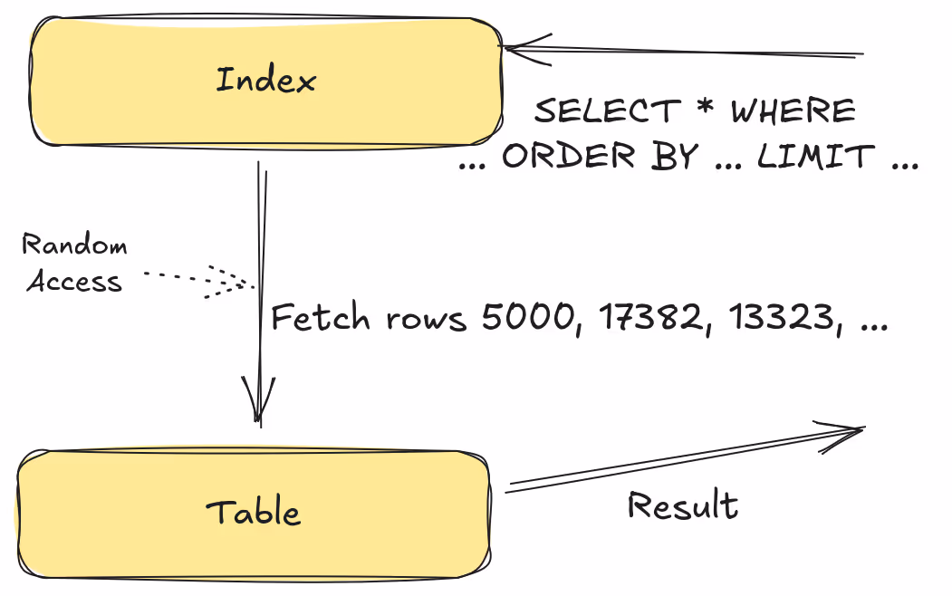
Vector search, text search, find-by-key, and key-based joins might seem like different problems but they all follow the same general process. Some kind of index structure is searched to figure out which rows match the query (or sometimes which rows might match the query). The return from this index search is a set of row ids. Next, we take those row ids and go fetch one or more columns for those rows. This is where the random access comes into play. Keeping these overall search use cases in mind helps us understand how to setup our benchmarks.

What we Benchmark

There are a lot of parameters that we can play with when benchmarking. If we try and tackle them all it could take ages. Instead we focus on the configuration most likely used by the use cases we encounter (as described above).

Metadata in Memory is the Common Case

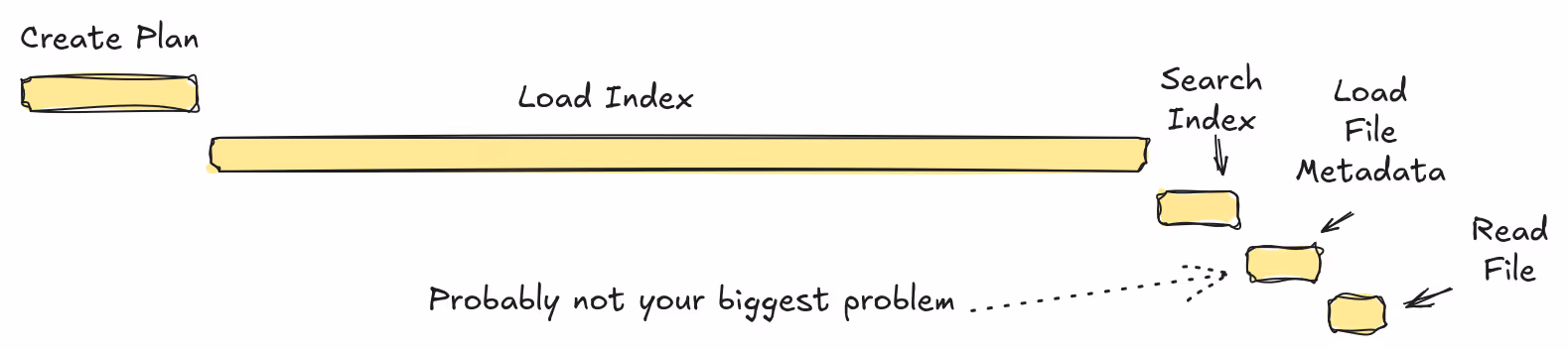
In order to satisfy a search we need to load the index, table metadata, file metadata, and finally the rows themselves. As latency is important in a search workload, we want to cache as much as possible. Lance will cache indexes, table metadata, and file metadata in memory by default. Lance does not do any caching of the rows themselves (we assume the actual row data is much larger than the available RAM and the kernel page cache is already doing a great job here). Because of this, our benchmarks usually assume the table and flie metadata are already loaded and cached in memory.

This doesn’t mean that “cold” searches (where there is nothing in the cache) are not a real use case. We have certain workload patterns where cold searches are very common and need to be optimized. For example, users that run Lance on some kind of transient compute that isn’t capable of caching anything in memory. However, when searches are cold, the latency is most likely going to be dominated by the index loading time. We definitely are not going to be reaching 1,000,000 IOPS with a cold search and so it isn’t a good use case for this blog post.

The Data Might not be Cached in Memory

Lance doesn’t do any caching of data. However, the kernel already does a great job of caching data itself. This can lead to a very common storage benchmarking blunder. Very few benchmarks bother to clear out the kernel cache and as a result they don’t actually measure the real world scenario. The benchmarks might be stellar but as soon as the working set for the data is much larger than the RAM on the machine the real-world performance and the benchmarking performance no longer align.

That being said, if we focus only on the not-in-cache case, we might get lazy for another reason. I/O is slow and we don’t notice the CPU bottlenecks because we have plenty of time. Then, when the working set does fit into memory, we are not achieving the best performance we could. As a result, most of our benchmarks consider both cases.

Consider Throughput in Addition to Latency

Another issue we see with a lot of benchmarking efforts is a focus on latency, rather than throughput. Latency is often a measure of how long it takes to run a single operation – for example, the end-to-end time of a single vector search or query. Throughput, on the other hand, measures how many operations we can measure in a given time period. If there were only a single core, then the two would be identical. If an operation takes X seconds then we can do 1/X operations per second.

What we’ve found when we measure throughput, and measure on multiple threads, is that something which gives us a boost to latency might actually interfere with throughput. This is typically related to thread synchronization overhead and processor cache contention. When we are testing one operation at a time then farming work onto additional threads is often a win. However, when measuring throughput, we can see that adding more tasks ends up degrading performance.

Batched Reads are Common

A simple benchmark might time how long it takes to read a single column from a single row. However, in practice, we are often reading not only multiple columns but also multiple rows. Consider a top-k search operation. After searching the index we have a set of rows that we need to go fetch. Lance supports this sort of batched read operation and we can amortize a lot of the small per-operation costs like scheduling, allocation, etc. We want to reflect this in our benchmarks and so we are typically fetching multiple rows at a time as part of the benchmark.

End-to-End Benchmarks » Micro Benchmarks

Micro benchmarks, focused on small portions of an operation, or those that focus on just the file format, are useful for profiling and regression and we have quite a few of them. However, it is entirely possible that what makes a micro benchmark perform well can actually hurt our end-to-end performance. When it comes to making technical decisions and setting good default configuration, we chiefly consider the end-to-end performance.

Putting it All Together (Incorrectly)

Now let’s tear apart the most common benchmark we see people run when they want to measure the random access performance of Lance (this might be a passive-aggressive exercise).

def bench_setup():
    indices = np.random.randint(0, 100_000_000, 1000)
    return indices

def bench_function(idx: int):
    ds = lance.dataset("path/to/dataset")
    ds.take([idx])

This is a simple benchmark but it fails pretty much all of our criteria. It has to reload all dataset metadata in each iteration. It’s purely focused on latency and does not consider thread synchronization overhead. The setup function is not clearing out the kernel page cache. It only reads a single row at a time.

The end result is that this benchmark isn’t really measuring what we actually do in the real world. In the next section I’ll describe the benchmarks I actually ran for this experiment.

The Quest for 1,000,000 IOPS

Now that we’ve got the groundwork established, let’s look at how that maps to our goal of 1,000,000 IOPS. The first thing I need to do is to find a way to convert this into an end-to-end benchmark. Vector search is one of our key use cases and so I chose that to work with initially. In future blog posts, I want to consider other cases, such as using LanceDB as a key-value store, or using LanceDB as a storage pushdown engine, but vector search is a good place to start.

Vector Search

To test out vector search performance I chose some numbers based on a recent use case from an integration partner. Generally, vector search is very compute intensive. So much so that I/O is not typically the bottleneck. However, this user wanted to run an I/O intensive vector search with just the scenario I needed. They wanted to search for the top 50 results but with a refine factor of 10. A refine factor multiplies the number of rows we need to fetch. So with a refine factor of 10 we will need to fetch 500 rows intead of 50. We then compare these 500 rows to our query vector to get the top 50.

As I mentioned earlier, we want to consider throughput in addition to latency. Having a low latency means the users are satisfied with the query performance. Having a high throughput means we can handle more queries per server and keeps our overall costs down. To achieve this in the benchmark I first set up a test dataset, then I generate a set of queries. Each query will fetch 500 rows so running 2,000 queries will fetch 1,000,000 rows. Now I start a worker for each thread, and each worker pulls queries from our queue and executes them. The queries are asynchronous. We have each thread run several queries at a time. Once all workers are finished we end the timer and report the results.

The benchmark code can be found on GitHub .

The Challenge

Before we get started, let’s understand the challenge here. We are trying to achieve 1,000,000 rows per second. That means that we will need to emit a single row every microsecond. To understand the challenge let’s look at napkin math . This is a simple tool to give us a sense of the scale of the problem. A single system call is ~500 nanoseconds. This is potentially tolerable. However, a random NVMe read is ~100 microseconds. This means we will need hundreds of concurrent reads to achieve our goal. Fortunately, I think the napkin math is a little off here. Specs for the drive say the latency for a read is more in the 10-20 microsecond range. Also, even if we do need hundreds of concurrent reads it doesn’t neccesarily mean hundreds of cores since the CPU can do work while waiting for I/O. A context switch is listed at ~10 microseconds. If every operation required a context switch then we’d need 10 cores just for context switching. Although if you have more cores you need more threads and if you have more theads you might get more context switches… Consider this foreshadowing for what is to come.

The moral of the story is that our CPU constraints are surprisingly tight, especially for something we might typically think of as I/O bound. We are going to need a considerable amount of parallelism in both the I/O and the CPU. At the same time, our tasks are fairly small, and we need to be sensitive to context switches and system calls.

Hardware

Our first problem is hardware. My development desktop has 16 cores (8 physical with hyperthreading) and a single NVMe drive that I can crank up to about 800,000 IOPS with fio. So off the bat we aren’t going to hit 1,000,000 IOPS with this hardware. That being said, I can do most of my experimentation on this machine with data cached in memory and extrapolate.

For the actual experiment I’m going to use an AWS i8g.12xlarge instance. This has 48 cores (24 physical with hyperthreading) and three NVMe drives, each with about 500K IOPS for a total of about 1.5M IOPS. This means I will need to spread my queries across three different datasets.

Starting Scores

To start with, let’s just run the benchmark and see what we get.

We are still a ways off from our goal but it’s a pretty solid start. For comparison, I designed a similar file-based benchmark that just does file reads against random rows. This allows us to compare Lance directly against file-only libraries like parquet-rs.

Unsurprisingly, we can see that Lance has already done quite a bit of optimization for this task. So our starting point is already about 5x that of parquet-rs, and we want to make it over twice as fast. We’re going to have to get into the fine details to reach our goal.

Phase 0: Tracing

I almost always start off profiling efforts with tracing. It’s very useful to understand what is actually happening and to get a broad overall sense of the costs. However, a lot of the issues we are going to be encountering today only show up at high scale and heavy load. I found tracing under these conditions to be either too broad (in which case it didn’t help narrow things down) or too detailed (in which case it impacted the results). In the end, I didn’t actually use tracing much in this experiment.

Phase 1: Flamegraphs

Flamegraphs are a great way to start. In this case, they help give a good visualization of the various CPU costs. Let’s take a look at the flamegraph from our benchmark.

This mostly makes sense. We are spending a lot of CPU time searching the vector index. The rest of the time is fairly evenly split among the various other tasks. There are some strange syscalls that aren’t reads which we will later learn are related to threading overhead.

First Conclusion: Index Search is Expensive

Searching a vector index is expensive. This is reflected in our flamegraph. I’ll save you the math, but we are not going to be able to hit our goal of 1,000,000 IOPS with this vector search configuration. We will revisit this later but for now we are just going to cheat. By dropping the nprobes parameter from 20 to 1 we can eliminate 95% of the work required by the index search. This isn’t free, it basically tanks our recall accuracy, but it lets us focus on the I/O. Later I will explain how we solve this problem at LanceDB so that we can have the best of both worlds but for now let’s just cheat.

As expected, the amount of time spent in the index search is much lower (10x). By removing 43% of the CPU work, we should expect the throughput to increase by about 1.75x. In reality it was a little closer to 1.5x. This could be another sign of synchronization overhead. It could also indicate some kind of I/O scheduling bottleneck. Even though our IOPS are well within the capabilities of the drive (we should be able to hit over 1,000 QPS on this drive), it’s possible we are not driving the disk correctly (e.g. not maintaining the proper queue depth). Still, we have reached 50 QPS/Core. If we scale up to our target system (48 cores) we should easily be able to hit our goal of 2,000 QPS. Let’s give it a try.

…

At this point, we’ve collected a number of interesting data points. They all seem to be pointing to a common culprit which is some kind of synchronization overhead or I/O bottleneck. In the next phase we are going to try and identify which of these is the actual culprit.

Phase 2: Pipelines

At this point we’ve exhausted our two traditional profiling tools, flamegraphs and tracing. There are dozens of other performance counters we can look at and, to be honest, I spent quite a bit of time looking at them, but I wouldn’t say I learned much. There is one last piece of evidence I wanted to collect before I started working on potential solutions. I wanted to look at the pipelines in the benchmark and verify my assumptions about which pipeline is the bottleneck.

Pipelines are a good vague word that can mean just about anything. For my purposes I’m going to define pipelines as a set of sequential steps with consistent parallelism (not neccesarily consistent partitioning). Our benchmark can be split into three pipelines:

1. Search & Schedule (CPU) - This is a pipeline where we figure out what rows we want by looking at the index. Then we look at table and file metadata to figure out where those rows are stored on disk. Finally, we issue the I/O requests for those rows.

2. Read (I/O) - Here we just read the data from the disk.

3. Decode (CPU) - Here we decode the data from the on-disk format into the desired in-memory layout of the data, rerank the results (this is part of the vector search) and return the results.

I’ve labeled the pipelines as CPU or I/O because this is what controls the parallelism of the pipeline. In our CPU pipelines we want to have one task per core. In our I/O pipelines the number of tasks is based on the number of concurrent I/O requests we can issue. For an NVMe drive this is partly a factor of the hardware (how many parallel components are available) and partly a factor of the OS (how many parallel I/O requests do we need to maintain the desired queue depth so that the drive is not starved)?

Another important note is that when we change parallelism, we also introduce a queue. The scheduling pipeline drops reads into a queue for the I/O pipeline. The I/O pipeline then drops the data into a queue for the decode pipeline. These queues can be valuable information for our performance analysis! Let’s run our benchmark again, but this time, let’s introduce instrumentation to track the size of the queues over time.

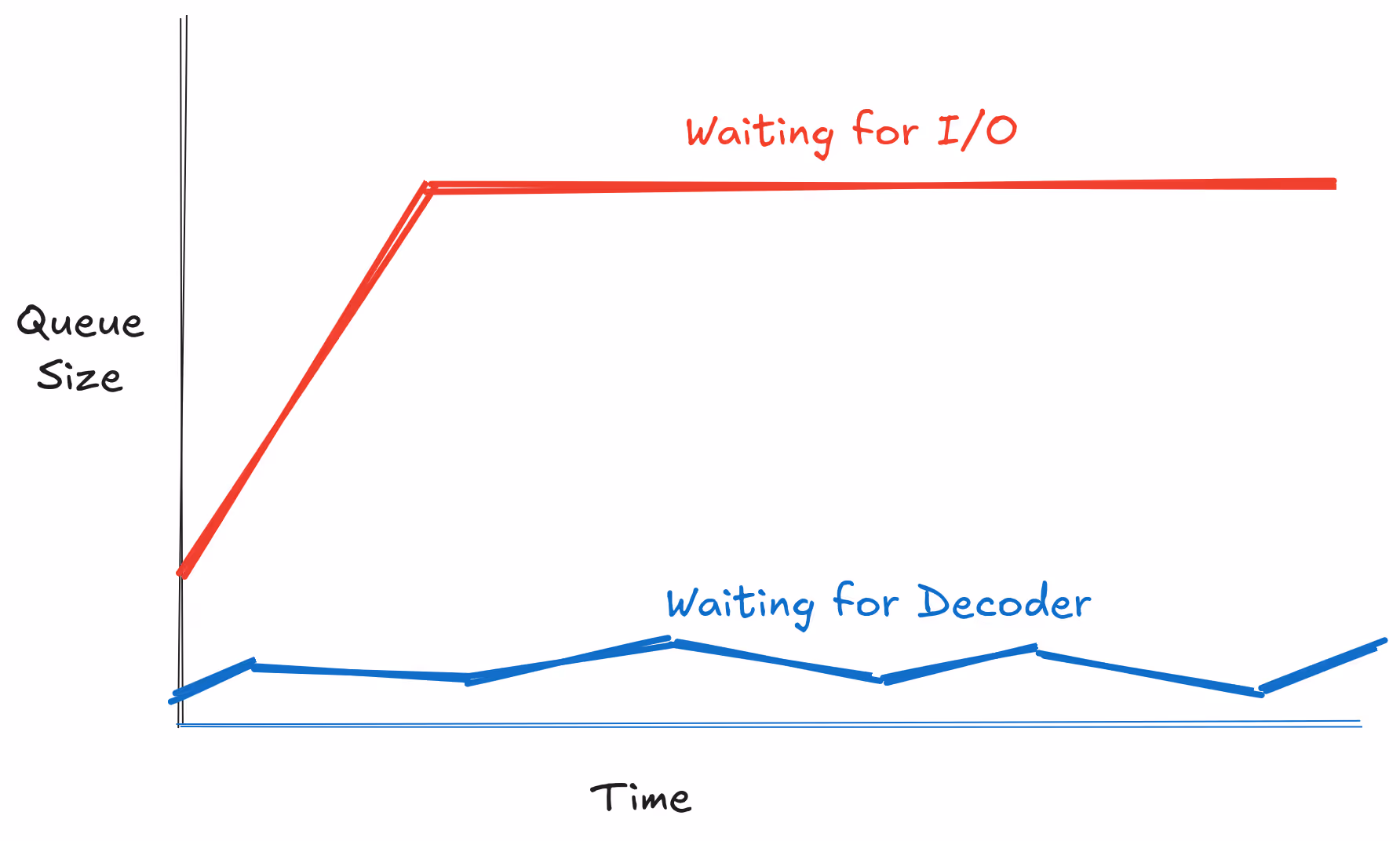
The I/O queue quickly fills up and hits capacity. Meanwhile, the decode queue bounces around but is generally near empty. This means our problem is now narrowed down to the I/O pipeline.

Solution 1: Scheduler Rework

Tracking down synchronization overhead can be a bit tricky. Traditional culprits of synchronization overhead are things like mutexes or condition variables. Our code (very intentionally) doesn’t actually have any of these. There is almost no writable shared state between queries. We have a few atomic counters for bookkeeping and the table and file metadata is in a shared LRU cache but the cache is hot and the critical section is a trivial arc copy and so there shouldn’t be any real contention here.

Other sources of contention include things like context switches and system calls (the Linux kernel is multithreaded but it has internal locks and critial sections of its own). Fortunately, profiling tools can measure all of these things. They provided some good insights into where to start and they detected a number of potential issues. The ones that ended up being most relevant were:

• Busy waiting in the tokio blocking thread pool
• Busy waiting in the tokio global thread pool
• System calls to park / unpark tokio tasks
• pread64 system calls

The first three items are all related to tokio, our favorite asynchronous runtime. To be clear, the problem is not a performance issue in tokio itself, but rather an issue with the way we were using it. To understand this issue, let’s take a closer look at what happens in the I/O pipeline. First, we place the request in a priority queue. This queue is where we enforce backpressure. Second, the I/O loop thread pulls items from the priority queue and issues the I/O requests. We are using pread64 which is a blocking system call. To interface this with tokio it means we need to launch a thread task on the blocking thread pool and so we enqueue a task. One of our blocking worker threads picks up the task and issues the system call. Once the system call completes we enqueue the results back into a queue for the decode pipeline.

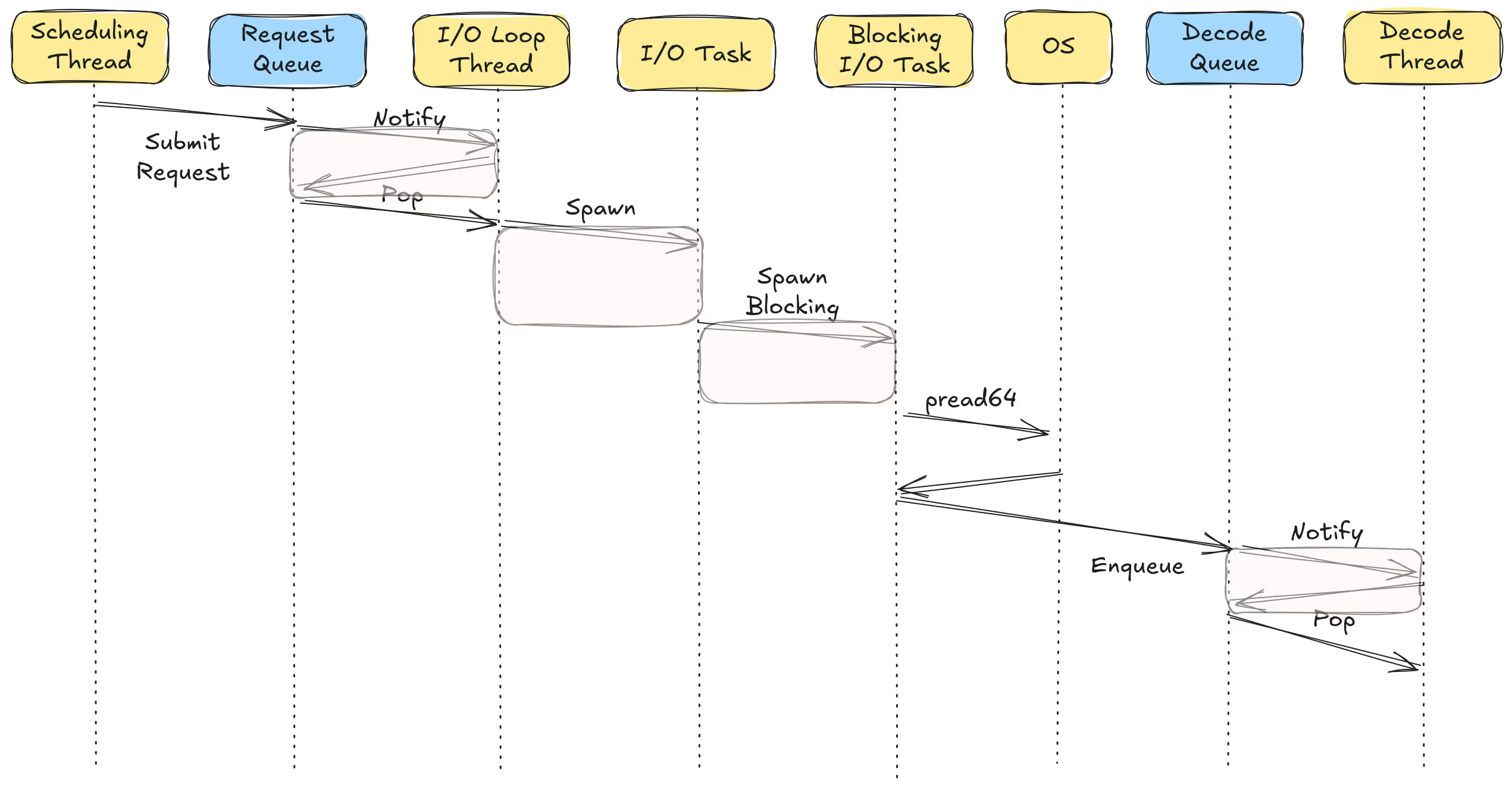
What all of this is doing is breaking our work up into smaller and smaller tasks. Switching between these tasks takes time and introduces overhead. Switching tasks is also a context switch (an asynchronous context switch in user space but still a context switch) which can mess up CPU cache locality (e.g. two sequential tasks might run on different cores). So our first fix is to rework the scheduler and reduce the number of tasks we are creating. The details are probably a bit too much for a blog post but the short version is that we got rid of a few ineffecient things and also sort of created our own tiny little event loop which, being very narrowly focused, avoids some of the overhead.

Results

Perhaps the most disheartening and frustrating part of this journey was the fact that this scheduler change had almost no effect on my desktop’s performance. I spent a lot of time debugging and tweaking things (see earlier aside on memory banwdith) and even when I ran it on the larger instance I didn’t see any real effect but this was because I was using I/O uring at this point and encountering a rather subtle bug in the scheduler (more on this later).

However, we have the benefit of hindsight, and so let’s take a look at the results (with the aforementioned bug fixed) on both systems.

Benchmarking Woes

Wait…have we done it?! We have over 2,000 queries per second on the AWS instance! Does this really mean we’ve hit 1,000,000 IOPS?

Sadly, no, we are not there yet. My initial excitement the first time I hit 2,000 QPS was premature and I wanted to drag you through the same experience because I’m a cruel storyteller. In order to independently verify our IOPS assumption we can use a tool called iostat. It prints out I/O statistics at a given interval. Running this on the above run we got the following results:

avg-cpu:  %user   %nice %system %iowait  %steal   %idle
          19.86    0.00   29.51    9.84    0.00   40.79

Device            r/s     rkB/s   rrqm/s  %rrqm r_await rareq-sz     w/s     wkB/s   wrqm/s  %wrqm w_await wareq-sz     d/s     dkB/s   drqm/s  %drqm d_await dareq-sz     f/s f_await  aqu-sz  %util
nvme0n1       198265.00 1311288.00     0.00   0.00    0.12     6.61    0.00      0.00     0.00   0.00    0.00     0.00    0.00      0.00     0.00   0.00    0.00     0.00    0.00    0.00   24.70  62.00
nvme1n1          0.00      0.00     0.00   0.00    0.00     0.00    0.00      0.00     0.00   0.00    0.00     0.00    0.00      0.00     0.00   0.00    0.00     0.00    0.00    0.00    0.00   0.00
nvme2n1       197704.00 1301960.00     0.00   0.00    0.12     6.59    0.00      0.00     0.00   0.00    0.00     0.00    0.00      0.00     0.00   0.00    0.00     0.00    0.00    0.00   24.38  62.10
nvme3n1       198417.00 1311072.00     0.00   0.00    0.12     6.61    0.00      0.00     0.00   0.00    0.00     0.00    0.00      0.00     0.00   0.00    0.00     0.00    0.00    0.00   22.92  62.30

Our three NVMe drives were definitely busy, but at our peak we only reached ~600,000 IOPS. After a fair amount of debugging I discovered that I was running into everyone’s favorite stasistical paradox, the birthday paradox. I created a test setup with one million vectors. Each vector is 3KiB and so requires at least some portion of its own 4KiB disk sector. I then issued a bunch of random queries. Many of the queries matched identical rows and so I wasn’t actually accessing 1,000,000 unique rows.

Luckily, the fix is simple, just use a larger dataset. Unfortunately, this means we have not quite reached our goal:

Solution 2: io_uring

By reworking the scheduler we were able to reduce the number of tasks a lot. However, we still have one blocking task and one system call for every single read. We can fix the first by batching reads together. Or, we can fix both by using io_uring which is an alternative kernel API for making I/O requests.

The io_uring API has a reputation for two things:

• Has a lot of cool optimizations which make I/O benchmarks very fast
• Not speeding up applications because it’s often misunderstood and/or misused

io_uring does not make I/O any faster. The benefits it delivers are primarily for CPU-bound or RAM-bound applications. This recent paper by does a good job of explaining the benefits. However, the main benefit we’re looking for here isn’t even really a benefit of the implementation itself. Rather, it’s simply having some kind of asynchronous API that allows us to reduce our task switching overhead. There are a lot of details I’m glossing over but I implemented io_uring for Lance and I settled on two different approaches.

Approach 1: Shared Rings

In this approach I create some small number of dedicated uring instances. When a request is submitted we pick a uring (using a basic round-robin approach) and submit the request to it via a queue. Each uring has its own dedicated thread that reads from the queue and processes the requests. This approach has the downside that we’re still breaking the work into smaller tasks. However, it has the advantage of being easy to use and has no requirements on the runtime, unlike our next approach.

Approach 2: Thread Local Runtime

In this second approach I create a single uring instance per thread. When a request is submitted we push it directly into the submission queue. Then, later, when the future is polled, we submit any requests and process completions. If there are no completions to process (I/O still in progress) then we yield. This yield is the only place in the entire I/O pipeline that could trigger an asynchronous context switch. We’ve collapsed the entire pipeline into a single task.

The disadvantage of this approach is that it requires all requests to be submitted from a single thread and it requires the decoder to be running on that same thread (since it polls the future). This is a tricky problem to solve when running in tokio but we’ve structured our benchmark in a way that we can handle it. If you’ll recall, our benchmark launches a number of current-thread runtimes which pull queries from a queue and runs them. Since each query is isolated to a single current-thread runtime we can rely on the entire query being processed on the same thread.

Results

The shared uring approach has an additional parameter which is the number of uring instances to use. More instances means we have higher CPU overhead (since the uring threads will spin whenever there is any I/O in progress) but higher throughput. For the uring per thread approach there are no additional parameters (and less overhead overall).

Both approaches are able to achieve roofline throughput. Also, to be clear, these scores are with the larger dataset. And just to double check:

avg-cpu:  %user   %nice %system %iowait  %steal   %idle
          46.81    0.00   29.50   18.75    0.00    4.95

Device            r/s     rkB/s   rrqm/s  %rrqm r_await rareq-sz     w/s     wkB/s   wrqm/s  %wrqm w_await wareq-sz     d/s     dkB/s   drqm/s  %drqm d_await dareq-sz     f/s f_await  aqu-sz  %util
nvme0n1       526327.00 3598392.00  7753.00   1.45    5.58     6.84    0.00      0.00     0.00   0.00    0.00     0.00    0.00      0.00     0.00   0.00    0.00     0.00    0.00    0.00 2938.26 100.00
nvme1n1          0.00      0.00     0.00   0.00    0.00     0.00    0.00      0.00     0.00   0.00    0.00     0.00    0.00      0.00     0.00   0.00    0.00     0.00    0.00    0.00    0.00   0.00
nvme2n1       523488.00 3575576.00  7692.00   1.45    4.14     6.83    0.00      0.00     0.00   0.00    0.00     0.00    0.00      0.00     0.00   0.00    0.00     0.00    0.00    0.00 2166.97 100.00
nvme3n1       523369.00 3583620.00  7639.00   1.44    3.39     6.85    0.00      0.00     0.00   0.00    0.00     0.00    0.00      0.00     0.00   0.00    0.00     0.00    0.00    0.00 1773.59  99.90

That’s right… 1,500,000 IOPS. Full disk utilization.

Just to put this in context, each vector is 3KiB and so this represents ~4.5GB/s of data being read from disk in completely random order. The actual number is quite a bit higher since disk sectors are 4KiB (not 3KiB) and our vectors aren’t aligned to disk sector boundaries. So most reads need to fetch 8KiB of data while some get away with 4KiB. This is why iostat is measuring ~10.5GB/s of data being read from disk.

Did the Scheduler Rework Matter?

An interesting question to ask is what would happen if we had just changed to using io_uring without the scheduler rework. Fortunately, we added the new scheduler alongside the old scheduler, so we can easily run the benchmark with io_uring and the old scheduler.

I find this result pretty fascinating. Adding io_uring by itself didn’t help performance at all. Adding the scheduler rework by itself only helped some. Adding both of them together truly gives us a “whole is greater than the sum of its parts” result.

Conclusions

• Single-read latency benchmarks are not a good proxy for understanding random access performance
• Fully utilizing NVMe drives requires a lot of attention to synchronization overhead
• By combining a scheduler rework with io_uring we were able to achieve 1,500,000 IOPS with Lance

What’s Next?

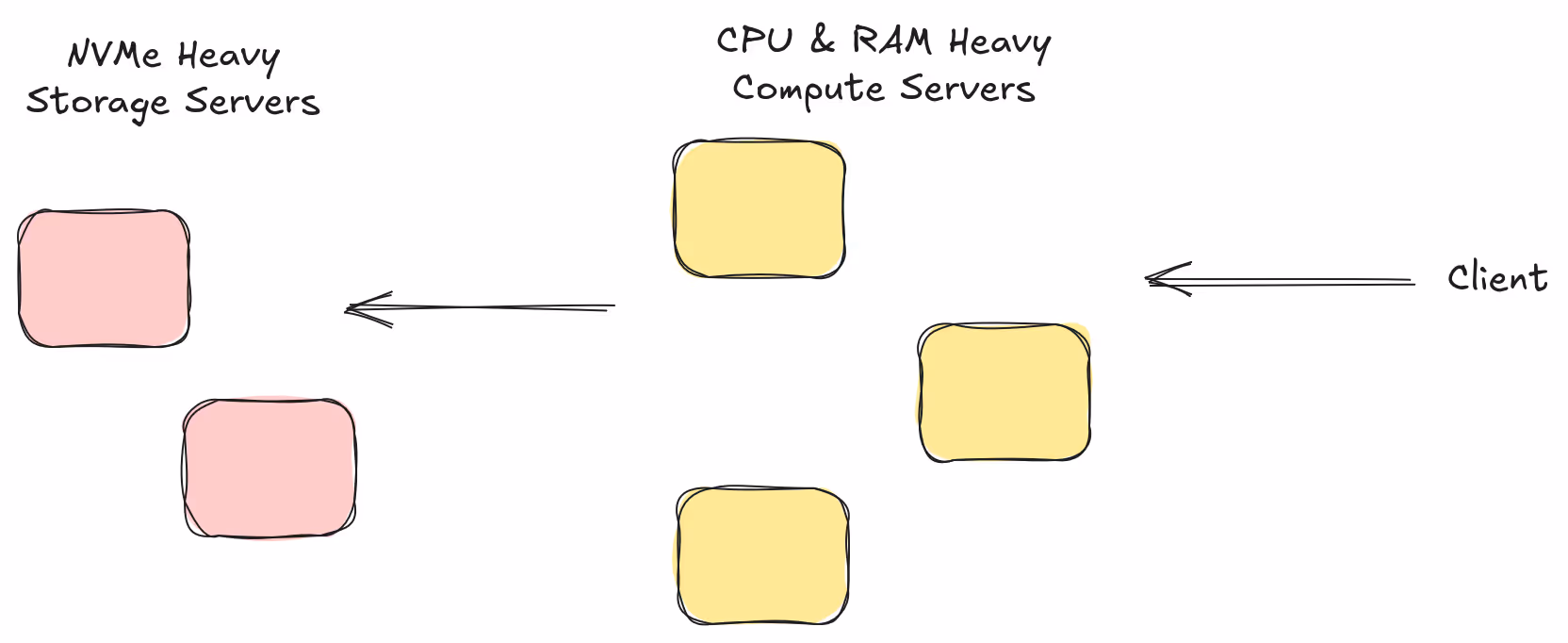
We’ve shown that we can achieve 1,000,000 IOPS in a vector search benchmark. However, if you recall, we had to cheat very early on in the process by reducing the nprobes from 20 to 1. This is going to generally give us some pretty terrible recall. In addition, the refine factor of 10 is pretty high. In other words, in most vector search applications, we are going to have a much more significant amount of CPU work to do in order to reach 1,000,000 IOPS. Fortunately, this is a problem we can solve, with the time honored tradition of compute-storage separation.

Lance is a format that can be deployed into a variety of architectures. By default, the OSS library LanceDB gives users an embedded database that runs everything in a single process. The architecture we use in our enterprise software actually separates the query stage from the I/O stage. When a query arrives we first search the index to find matching row ids. We then send those row ids to another server to fetch them from the disk. This allows us to scale up our query nodes to meet the demands of the index search (Do we need high recall? Is there expensive prefiltering?) while independently scaling high-throughput I/O nodes to meet the demands of the data access. In a future benchmark I hope to explore the 1,000,000 IOPS goal with this architecture (e.g. can I build an NVMe caching service that can achieve 1,000,000 IOPS?)

Before I get there however I also want to take a look at a different workflow, the key-value store workflow. In this workflow users are often fetching a very small number of rows (typically just one) but expect a very high number of queries per second (ideally, 1,000,000). To achieve 1,000,000 QPS we are going to face a slightly different set of challenges and I’m hoping to explore those in a future blog post.